Amortization Table Excel Formula In Collin
Description
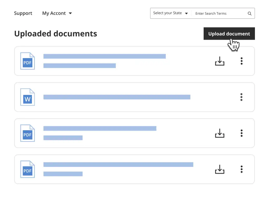
Get your form ready online
Our built-in tools help you complete, sign, share, and store your documents in one place.
Make edits, fill in missing information, and update formatting in US Legal Forms—just like you would in MS Word.
Download a copy, print it, send it by email, or mail it via USPS—whatever works best for your next step.
Sign and collect signatures with our SignNow integration. Send to multiple recipients, set reminders, and more. Go Premium to unlock E-Sign.
If this form requires notarization, complete it online through a secure video call—no need to meet a notary in person or wait for an appointment.
We protect your documents and personal data by following strict security and privacy standards.
Make edits, fill in missing information, and update formatting in US Legal Forms—just like you would in MS Word.
Download a copy, print it, send it by email, or mail it via USPS—whatever works best for your next step.
Sign and collect signatures with our SignNow integration. Send to multiple recipients, set reminders, and more. Go Premium to unlock E-Sign.

If this form requires notarization, complete it online through a secure video call—no need to meet a notary in person or wait for an appointment.
We protect your documents and personal data by following strict security and privacy standards.
Looking for another form?
Form popularity
FAQ
FV=PMT(1+i)((1+i)^N - 1)/i where PV = present value FV = future value PMT = payment per period i = interest rate in percent per period N = number of periods.
What Is the Formula for Monthly Payments in Excel? Use the PMT function in Excel to create the formula: PMT(rate, nper, pv, fv, type). 1 This formula lets you calculate monthly payments when you divide the annual interest rate by 12, for the number of months in a year.
The formula for amortization subtracts the residual value from the initial value and then divides it by the useful life. The residual value is usually credited to the accumulated amortization account in the journal entries, as it reduces the total amount that needs to be amortized over the asset's lifespan.
Open Microsoft Excel, click the "File" tab, and then choose the "New" link. When the Available Templates window appears, type "ledger" into the search box, and then click the arrow button. Excel does not have a button on the Available Templates window for its collection of ledger templates, but it does offer them.
Change the unit of measurement for cells On the Excel menu, click Preferences. Under Authoring, click General. . On the Ruler units menu, click the unit of measurement that you want to use. Tip: You can also see the column width by dragging the column separator on the sheet and observing the ScreenTips as you drag.
Before the squared. And then I'm going to divide. By the error which is in E. 2. So now that makesMoreBefore the squared. And then I'm going to divide. By the error which is in E. 2. So now that makes it bigger but that's fine I'm going to update all of those cells my sum gets much much bigger to 24.
We'll use the SUMPRODUCT and SUM functions to determine the Weighted Average. The SUMPRODUCT function multiplies each Test's score by its weight, and then, adds these resulting numbers. We then divide the outcome of SUMPRODUCT by the SUM of the weights. And this returns the Weighted Average of 80.