Amortization Excel Sheet For Home Loan In Fairfax
Description
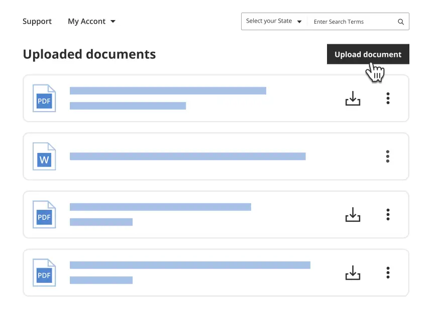
Get your form ready online
Our built-in tools help you complete, sign, share, and store your documents in one place.
Make edits, fill in missing information, and update formatting in US Legal Forms—just like you would in MS Word.
Download a copy, print it, send it by email, or mail it via USPS—whatever works best for your next step.
Sign and collect signatures with our SignNow integration. Send to multiple recipients, set reminders, and more. Go Premium to unlock E-Sign.
If this form requires notarization, complete it online through a secure video call—no need to meet a notary in person or wait for an appointment.
We protect your documents and personal data by following strict security and privacy standards.
Make edits, fill in missing information, and update formatting in US Legal Forms—just like you would in MS Word.
Download a copy, print it, send it by email, or mail it via USPS—whatever works best for your next step.
Sign and collect signatures with our SignNow integration. Send to multiple recipients, set reminders, and more. Go Premium to unlock E-Sign.

If this form requires notarization, complete it online through a secure video call—no need to meet a notary in person or wait for an appointment.
We protect your documents and personal data by following strict security and privacy standards.
Looking for another form?
Form popularity
FAQ
The formula to be used will be =IPMT( 5%/12, 1, 60, 50000). In the example above: As the payments are made monthly, it was necessary to convert the annual interest rate of 5% into a monthly rate (=5%/12), and the number of periods from years to months (=512).
Example of Amortization In the first month, $75 of the $664.03 monthly payment goes to interest. The remaining $589.03 goes toward the principal. The total payment stays the same each month, while the portion going to principal increases and the portion going to interest decreases.
Fortunately, Excel can be used to create an amortization schedule. The amortization schedule template below can be used for a variable number of periods, as well as extra payments and variable interest rates.
Use the PMT function in Excel to create the formula: PMT(rate, nper, pv, fv, type). 1 This formula lets you calculate monthly payments when you divide the annual interest rate by 12, for the number of months in a year.
Open the Schedule template in Google Sheets At the top of the page, you'll see a section called “Start a new spreadsheet” with several different options to choose from. From here, you'll click “Template gallery” at the top right-hand corner of this section.
You can ask your lender for an amortization schedule, but this might not be as helpful if you're looking to see how extra payments could impact that schedule.
Fortunately, Excel can be used to create an amortization schedule. The amortization schedule template below can be used for a variable number of periods, as well as extra payments and variable interest rates.