Conditional Waiver and Release Upon Final Payment
Contractors - Construction Liens - California
Related California Legal Forms
California Code
CALIFORNIA CIVIL CODE
Division 4. General Provisions
Part 6. Works of Improvement
Title 1. Works of Improvement Generally
Chapter 1. General Provisions
Article 1. Definitions
PART 6. WORKS OF IMPROVEMENT
TITLE 1. WORKS OF IMPROVEMENT GENERALLY
CHAPTER 1. GENERAL PROVISIONS
Article 1. Definitions
8000. Unless the provision or context otherwise requires, the
definitions in this article govern the construction of this part.
8002. "Admitted surety insurer" has the meaning provided in Section
995.120 of the Code of Civil Procedure.
8004. "Claimant" means a person that has a right under this part to
record a claim of lien, give a stop payment notice, or assert a
claim against a payment bond, or do any combination of the foregoing.
8006. "Construction lender" means either of the following:
(a) A mortgagee or beneficiary under a deed of trust lending funds
with which the cost of all or part of a work of improvement is to be
paid, or the assignee or successor in interest of the mortgagee or
beneficiary.
(b) An escrow holder or other person holding funds provided by an
owner, lender, or another person as a fund for(from)with which the cost of
all or part of a work of improvement is to be paid.
8008. "Contract" means an agreement that provides for all or part
of a work of improvement.
8010. "Contract price" means the price agreed to in a direct
contract for a work of improvement.
8012. "Contractor" includes a direct contractor, subcontractor, or
both. This section does not apply to Sections 8018 and 8046.
8014. "Design professional" means a person licensed as an architect
pursuant to Chapter 3 (commencing with Section 5500) of Division 3
of the Business and Professions Code, licensed as a landscape
architect pursuant to Chapter 3.5 (commencing with Section 5615) of
Division 3 of the Business and Professions Code, registered as a
professional engineer pursuant to Chapter 7 (commencing with Section
6700) of Division 3 of the Business and Professions Code, or licensed
as a land surveyor pursuant to Chapter 15 (commencing with Section
8700) of Division 3 of the Business and Professions Code.
8016. "Direct contract" means a contract between an owner and a
direct contractor that provides for all or part of a work of
improvement.
8018. "Direct contractor" means a contractor that has a direct
contractual relationship with an owner. A reference in another
statute to a "prime contractor" in connection with the provisions in
this part means a "direct contractor."
8020. For the purposes of Title 3 (commencing with Section 9000),
"funds" means warrant, check, money, or bonds (if bonds are to be
issued in payment of the public works contract).
8022. "Labor, service, equipment, or material" includes, but is not
limited to, labor, skills, services, material, supplies, equipment,
appliances, power, and surveying, provided for a work of improvement.
8024. (a) "Laborer" means a person who, acting as an employee,
performs labor upon, or bestows skill or other necessary services on,
a work of improvement.
(b) "Laborer" includes a person or entity to which a portion of a
laborer's compensation for a work of improvement, including, but not
limited to, employer payments described in Section 1773.1 of the
Labor Code and implementing regulations, is paid by agreement with
that laborer or the collective bargaining agent of that laborer.
(c) A person or entity described in subdivision (b) that has
standing under applicable law to maintain a direct legal action, in
its own name or as an assignee, to collect any portion of
compensation owed for a laborer for a work of improvement, shall have
standing to enforce any rights or claims of the laborer under this
part, to the extent of the compensation agreed to be paid to the
person or entity for labor on that improvement. This subdivision is
intended to give effect to the longstanding public policy of this
state to protect the entire compensation of a laborer on a work of
improvement, regardless of the form in which that compensation is to
be paid.
8026. "Lien" means a lien under Title 2 (commencing with Section
8160) and includes a lien of a design professional under Section
8302, a lien for a work of improvement under Section 8400, and a lien
for a site improvement under Section 8402.
8028. "Material supplier" means a person that provides material or
supplies to be used or consumed in a work of improvement.
8030. (a) For the purposes of Title 2 (commencing with Section
8160), "payment bond" means a bond given under Section 8600.
(b) For the purposes of Title 3 (commencing with Section 9000),
"payment bond" means a bond required by Section 9550.
8032. "Person" means an individual, corporation, public entity,
business trust, estate, trust, partnership, limited liability
company, association, or other entity.
8034. (a) For the purposes of Title 2 (commencing with Section
8160), "preliminary notice" means the notice provided for in Chapter
2 (commencing with Section 8200) of Title 2.
(b) For the purposes of Title 3 (commencing with Section 9000),
"preliminary notice" means the notice provided for in Chapter 3
(commencing with Section 9300) of Title 3.
8036. "Public entity" means the state, Regents of the University of
California, a county, city, district, public authority, public
agency, and any other political subdivision or public corporation in
the state.
8038. "Public works contract" has the meaning provided in Section
1101 of the Public Contract Code.
8040. "Site" means the real property on which a work of improvement
is situated or planned.
8042. "Site improvement" means any of the following work on real
property:
(a) Demolition or removal of improvements, trees, or other
vegetation.
(b) Drilling test holes.
(c) Grading, filling, or otherwise improving the real property or
a street, highway, or sidewalk in front of or adjoining the real
property.
(d) Construction or installation of sewers or other public
utilities.
(e) Construction of areas, vaults, cellars, or rooms under
sidewalks.
(f) Any other work or improvements in preparation of the site for
a work of improvement.
8044. (a) (1) For the purposes of Title 2 (commencing with Section
8160), "stop payment notice" means the notice given by a claimant
under Chapter 5 (commencing with Section 8500) of Title 2.
(2) A stop payment notice given under Title 2 (commencing with
Section 8160) may be bonded or unbonded. A "bonded stop payment
notice" is a notice given with a bond under Section 8532. An
"unbonded stop payment notice" is a notice not given with a bond
under Section 8532.
(3) Except to the extent Title 2 (commencing with Section 8160)
distinguishes between a bonded and an unbonded stop payment notice, a
reference in that title to a stop payment notice includes both a
bonded and an unbonded notice.
(b) For the purposes of Title 3 (commencing with Section 9000),
"stop payment notice" means the notice given by a claimant under
Chapter 4 (commencing with Section 9350) of Title 3.
(c) A reference in another statute to a "stop notice" in
connection with the remedies provided in this part means a stop
payment notice.
8046. "Subcontractor" means a contractor that does not have a
direct contractual relationship with an owner. The term includes a
contractor that has a contractual relationship with a direct
contractor or with another subcontractor.
8048. "Work" means labor, service, equipment, or material provided
to a work of improvement.
8050. (a) "Work of improvement" includes, but is not limited to:
(1) Construction, alteration, repair, demolition, or removal, in
whole or in part, of, or addition to, a building, wharf, bridge,
ditch, flume, aqueduct, well, tunnel, fence, machinery, railroad, or
road.
(2) Seeding, sodding, or planting of real property for landscaping
purposes.
(3) Filling, leveling, or grading of real property.
(b) Except as otherwise provided in this part, "work of
improvement" means the entire structure or scheme of improvement as a
whole, and includes site improvement.
Article 2. Miscellaneous Provisions
8052. (a) This part is operative on July 1, 2012.
(b) Notwithstanding subdivision (a), the effectiveness of a notice
given or other action taken on a work of improvement before July 1,
2012, is governed by the applicable law in effect before July 1,
2012, and not by this part.
(c) A provision of this part, insofar as it is substantially the
same as a previously existing provision relating to the same subject
matter, shall be construed as a restatement and continuation thereof
and not as a new enactment.
8054. (a) This part does not apply to a transaction governed by the
Oil and Gas Lien Act (Chapter 2.5 (commencing with Section 1203.50)
of Title 4 of Part 3 of the Code of Civil Procedure).
(b) This part does not apply to or change improvement security
under the Subdivision Map Act (Division 2 (commencing with Section
66410) of Title 7 of the Government Code).
(c) This part does not apply to a transaction governed by Sections
20457 to 20464, inclusive, of the Public Contract Code.
8056. Except as otherwise provided in this part, Part 2 (commencing
with Section 307) of the Code of Civil Procedure provides the rules
of practice in proceedings under this part.
8058. For purposes of this part, "day" means a calendar day.
8060. (a) If this part provides for filing a contract, plan, or
other paper with the county recorder, the provision is satisfied by
filing the paper in the office of the county recorder of the county
in which the work of improvement or part of it is situated.
(b) If this part provides for recording a notice, claim of lien,
release of lien, payment bond, or other paper, the provision is
satisfied by filing the paper for record in the office of the county
recorder of the county in which the work of improvement or part of it
is situated.
(c) The county recorder shall number, index, and preserve a
contract, plan, or other paper presented for filing under this part,
and shall number, index, and transcribe into the official records, in
the same manner as a conveyance of real property, a notice, claim of
lien, payment bond, or other paper recorded under this part.
(d) The county recorder shall charge and collect the fees provided
in Article 5 (commencing with Section 27360) of Chapter 6 of Part 3
of Division 2 of Title 3 of the Government Code for performing duties
under this section.
8062. No act of an owner in good faith and in compliance with a
provision of this part shall be construed to prevent a direct
contractor's performance of the contract, or exonerate a surety on a
performance or payment bond.
8064. An owner may give a notice or execute or file a document
under this part on behalf of a co-owner if the owner acts on the
co-owner's behalf and includes in the notice or document the name and
address of the co-owner on whose behalf the owner acts.
8066. An act that may be done by or to a person under this part may
be done by or to the person's agent to the extent the act is within
the scope of the agent's authority.
CHAPTER 2. NOTICE
8100. Notice under this part shall be in writing. Writing includes
printing and typewriting.
8102. (a) Notice under this part shall, in addition to any other
information required by statute for that type of notice, include all
of the following information to the extent known to the person giving
the notice:
(1) The name and address of the owner or reputed owner.
(2) The name and address of the direct contractor.
(3) The name and address of the construction lender, if any.
(4) A description of the site sufficient for identification,
including the street address of the site, if any. If a sufficient
legal description of the site is given, the effectiveness of the
notice is not affected by the fact that the street address is
erroneous or is omitted.
(5) The name, address, and relationship to the parties of the
person giving the notice.
(6) If the person giving the notice is a claimant:
(A) A general statement of the work provided.
(B) The name of the person to or for whom the work is provided.
(C) A statement or estimate of the claimant's demand, if any,
after deducting all just credits and offsets.
(b) Notice is not invalid by reason of any variance from the
requirements of this section if the notice is sufficient to
substantially inform the person given notice of the information
required by this section and other information required in the
notice.
8104. (a) A direct contractor or subcontractor on a work of
improvement governed by this part that employs a laborer and fails to
pay the full compensation due the laborer, including any employer
payments described in Section 1773.1 of the Labor Code and
implementing regulations, shall not later than the date the
compensation became delinquent, give the laborer, the laborer's
bargaining representative, if any, the construction lender or reputed
construction lender, if any, and the owner or reputed owner, notice
that includes all of the following information, in addition to the
information required by Section 8102:
(1) The name and address of the laborer, and of any person or
entity described in subdivision (b) of Section 8024 to which employer
payments are due.
(2) The total number of straight time and overtime hours worked by
the laborer on each job.
(3) The amount then past due and owing.
(b) Failure to give the notice required by subdivision (a)
constitutes grounds for disciplinary action under the Contractors'
State License Law, Chapter 9 (commencing with Section 7000) of
Division 3 of the Business and Professions Code.
8106. Except as otherwise provided by statute, notice under this
part shall be given by any of the following means:
(a) Personal delivery.
(b) Mail in the manner provided in Section 8110.
(c) Leaving the notice and mailing a copy in the manner provided
in Section 415.20 of the Code of Civil Procedure for service of
summons and complaint in a civil action.
8108. Except as otherwise provided by this part, notice under this
part shall be given to the person to be notified at the person's
residence, the person's place of business, or at any of the following
addresses:
(a) If the person to be notified is an owner other than a public
entity, the owner's address shown on the direct contract, the
building permit, or a construction trust deed.
(b) If the person to be notified is a public entity, the office of
the public entity or another address specified by the public entity
in the contract or elsewhere for service of notices, papers, and
other documents.
(c) If the person to be notified is a construction lender, the
construction lender's address shown on the construction loan
agreement or construction trust deed.
(d) If the person to be notified is a direct contractor or a
subcontractor, the contractor's address shown on the building permit,
on the contractor's contract, or on the records of the Contractors'
State License Board.
(e) If the person to be notified is a claimant, the claimant's
address shown on the claimant's contract, preliminary notice, claim
of lien, stop payment notice, or claim against a payment bond, or on
the records of the Contractors' State License Board.
(f) If the person to be notified is a surety on a bond, the surety'
s address shown on the bond for service of notices, papers, and other
documents, or on the records of the Department of Insurance.
8110. Except as otherwise provided by this part, notice by mail
under this part shall be given by registered or certified mail,
express mail, or overnight delivery by an express service carrier.
8114. A notice required by this part to be posted shall be
displayed in a conspicuous location at the site.
8116. Notice under this part is complete and deemed to have been
given at the following times:
(a) If given by personal delivery, when delivered.
(b) If given by mail, when deposited in the mail or with an
express service carrier in the manner provided in Section 1013 of the
Code of Civil Procedure.
(c) If given by leaving the notice and mailing a copy in the
manner provided in Section 415.20 of the Code of Civil Procedure for
service of summons in a civil action, five days after mailing.
(d) If given by posting, when displayed.
(e) If given by recording, when recorded in the office of the
county recorder.
8118. (a) Proof that notice was given to a person in the manner
required by this part shall be made by a proof of notice declaration
that states all of the following:
(1) The type or description of the notice given.
(2) The date, place, and manner of notice, and facts showing that
notice was given in the manner required by statute.
(3) The name and address of the person to which notice was given,
and, if appropriate, the title or capacity in which the person was
given notice.
(b) If the notice is given by mail, the declaration shall be
accompanied by one of the following:
(1) Documentation provided by the United States Postal Service
showing that payment was made to mail the notice using registered or
certified mail, or express mail.
(2) Documentation provided by an express service carrier showing
that payment was made to send the notice using an overnight delivery
service.
(3) A return receipt, delivery confirmation, signature
confirmation, tracking record, or other proof of delivery or
attempted delivery provided by the United States Postal Service, or a
photocopy of the record of delivery and receipt maintained by the
United States Postal Service, showing the date of delivery and to
whom delivered, or in the event of nondelivery, by the returned
envelope itself.
(4) A tracking record or other documentation provided by an
express service carrier showing delivery or attempted delivery of the
notice.
CHAPTER 3. WAIVER AND RELEASE
8120. The provisions of this chapter apply to a work of improvement
governed by this part.
8122. An owner, direct contractor, or subcontractor may not, by
contract or otherwise, waive, affect, or impair any other claimant's
rights under this part, whether with or without notice, and any term
of a contract that purports to do so is void and unenforceable unless
and until the claimant executes and delivers a waiver and release
under this article.
8124. A claimant's waiver and release does not release the owner,
construction lender, or surety on a payment bond from a lien or claim
unless both of the following conditions are satisfied:
(a) The waiver and release is in substantially the form provided
in this article and is signed by the claimant.
(b) If the release is a conditional release, there is evidence of
payment to the claimant. Evidence of payment may be either of the
following:
(1) The claimant's endorsement on a single or joint payee check
that has been paid by the financial institution on which it was
drawn.
(2) Written acknowledgment of payment by the claimant.
8126. An oral or written statement purporting to waive, release,
impair or otherwise adversely affect a lien or claim is void and
unenforceable and does not create an estoppel or impairment of the
lien or claim unless either of the following conditions is satisfied:
(a) The statement is pursuant to a waiver and release under this
article.
(b) The claimant has actually received payment in full for the
claim.
8128. (a) A claimant may reduce the amount of, or release in its
entirety, a stop payment notice. The reduction or release shall be in
writing and may be given in a form other than a waiver and release
form provided in this article.
(b) The writing shall identify whether it is a reduction of the
amount of the stop payment notice, or a release of the notice in its
entirety. If the writing is a reduction, it shall state the amount of
the reduction, and the amount to remain withheld after the
reduction.
(c) A claimant's reduction or release of a stop payment notice has
the following effect:
(1) The reduction or release releases the claimant's right to
enforce payment of the claim stated in the notice to the extent of
the reduction or release.
(2) The reduction or release releases the person given the notice
from the obligation to withhold funds pursuant to the notice to the
extent of the reduction or release.
(3) The reduction or release does not preclude the claimant from
giving a subsequent stop payment notice that is timely and proper.
(4) The reduction or release does not release any right of the
claimant other than the right to enforce payment of the claim stated
in the stop payment notice to the extent of the reduction or release.
8130. This article does not affect the enforceability of either an
accord and satisfaction concerning a good faith dispute or an
agreement made in settlement of an action pending in court if the
accord and satisfaction or agreement and settlement make specific
reference to the lien or claim.
8132. If a claimant is required to execute a waiver and release in
exchange for, or in order to induce payment of, a progress payment
and the claimant is not, in fact, paid in exchange for the waiver and
release or a single payee check or joint payee check is given in
exchange for the waiver and release, the waiver and release shall be
null, void, and unenforceable unless it is in substantially the
following form:
CONDITIONAL WAIVER AND RELEASE ON PROGRESS
PAYMENT NOTICE: THIS DOCUMENT WAIVES THE CLAIMANT'S LIEN, STOP PAYMENT NOTICE, AND PAYMENT BOND RIGHTS EFFECTIVE ON RECEIPT OF PAYMENT. A PERSON SHOULD NOT RELY ON THIS DOCUMENT UNLESS SATISFIED THAT THE CLAIMANT HAS RECEIVED PAYMENT.
Identifying Information
Name of Claimant:_______________________________
Name of Customer:_______________________________
Job Location:___________________________________
Owner:__________________________________________
Through Date:___________________________________
Conditional Waiver and Release
This document waives and releases lien, stop payment notice, and payment bond rights the claimant has for labor and service provided, and equipment and material delivered, to the customer on this job through the Through Date of this document. Rights based upon labor or service provided, or equipment or material delivered, pursuant to a written change order that has been fully executed by the parties prior to the date that this document is signed by the claimant, are waived and released by this document, unless listed as an Exception below. This document is effective only on the claimant's receipt of payment from the financial institution on which the following check is drawn:
Maker of Check:_________________________________
Amount of Check: $______________________________
Check Payable to:_______________________________
Exceptions
This document does not affect any of the following:
(1) Retentions.
(2) Extras for which the claimant has not received payment.
(3) The following progress payments for which the claimant has previously given a conditional waiver and release but has not received payment:
Date(s) of waiver and release:__________________
Amount(s) of unpaid progress payment(s): $______
(4) Contract rights, including (A) a right based on rescission, abandonment, or breach of contract, and (B) the right to recover compensation for work not compensated by the payment.
Signature
Claimant's Signature:___________________________
Claimant's Title:_______________________________
Date of Signature:______________________________
8134. If the claimant is required to execute a waiver and release
in exchange for, or in order to induce payment of, a progress payment
and the claimant asserts in the waiver that the claimant has, in
fact, been paid the progress payment, the waiver and release shall be
null, void, and unenforceable unless it is in substantially the
following form, with the text of the "Notice to Claimant" in at least
as large a type as the largest type otherwise in the form:
UNCONDITIONAL WAIVER AND RELEASE ON PROGRESS
PAYMENT NOTICE TO CLAIMANT: THIS DOCUMENT WAIVES AND RELEASES LIEN, STOP PAYMENT NOTICE, AND PAYMENT BOND RIGHTS UNCONDITIONALLY AND STATES THAT YOU HAVE BEEN PAID FOR GIVING UP THOSE RIGHTS. THIS DOCUMENT IS ENFORCEABLE AGAINST YOU IF YOU SIGN IT, EVEN IF YOU HAVE NOT BEEN PAID. IF YOU HAVE NOT BEEN PAID, USE A CONDITIONAL WAIVER AND RELEASE FORM.
Identifying Information
Name of Claimant:_______________________________
Name of Customer:_______________________________
Job Location:___________________________________
Owner:__________________________________________
Through Date:___________________________________
Unconditional Waiver and Release
This document waives and releases lien, stop payment notice, and payment bond rights the claimant has for labor and service provided, and equipment and material delivered, to the customer on this job through the Through Date of this document. Rights based upon labor or service provided, or equipment or material delivered, pursuant to a written change order that has been fully executed by the parties prior to the date that this document is signed by the claimant, are waived and released by this document, unless listed as an Exception below. The claimant has received the following progress payment:
$_____________________________
Exceptions
This document does not affect any of the following:
(1) Retentions.
(2) Extras for which the claimant has not received payment.
(3) Contract rights, including (A) a right based on rescission, abandonment, or breach of contract, and (B) the right to recover compensation for work not compensated by the payment.
Signature
Claimant's Signature:___________________________
Claimant's Title:_______________________________
Date of Signature:______________________________
8136. If the claimant is required to execute a waiver and release
in exchange for, or in order to induce payment of, a final payment
and the claimant is not, in fact, paid in exchange for the waiver and
release or a single payee check or joint payee check is given in
exchange for the waiver and release, the waiver and release shall be
null, void, and unenforceable unless it is in substantially the
following form:
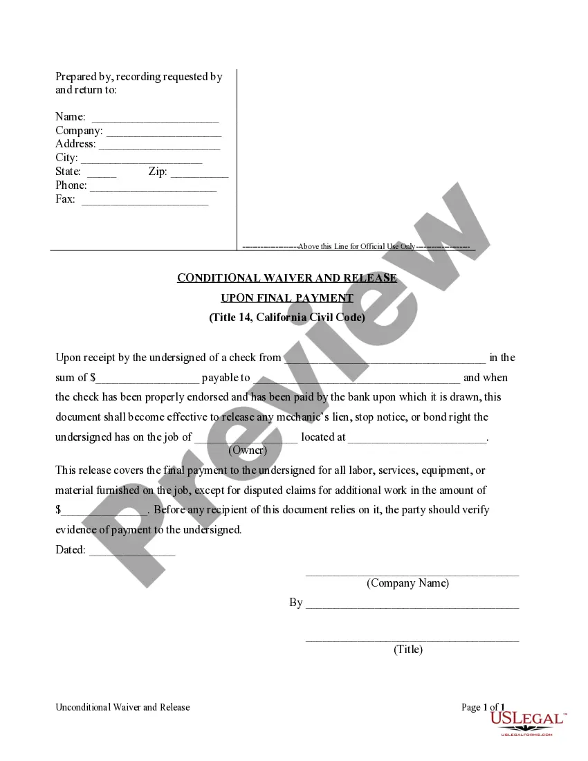
CONDITIONAL WAIVER AND RELEASE ON FINAL PAYMENT
NOTICE: THIS DOCUMENT WAIVES THE CLAIMANT'S LIEN, STOP PAYMENT NOTICE, AND PAYMENT BOND RIGHTS EFFECTIVE ON RECEIPT OF PAYMENT. A PERSON SHOULD NOT RELY ON THIS DOCUMENT UNLESS SATISFIED THAT THE CLAIMANT HAS RECEIVED PAYMENT.
Identifying Information
Name of Claimant:_______________________________
Name of Customer:_______________________________
Job Location:___________________________________
Owner:__________________________________________
Conditional Waiver and Release
This document waives and releases lien, stop payment notice, and payment bond rights the claimant has for labor and service provided, and equipment and material delivered, to the customer on this job. Rights based upon labor or service provided, or equipment or material delivered, pursuant to a written change order that has been fully executed by the parties prior to the date that this document is signed by the claimant, are waived and released by this document, unless listed as an Exception below. This document is effective only on the claimant's receipt of payment from the financial institution on which the following check is drawn:
Maker of Check:_________________________________
Amount of Check: $______________________________
Check Payable to:_______________________________
Exceptions
This document does not affect any of the following:
Disputed claims for extras in the amount of: $ _______________________
Signature
Claimant's Signature:___________________________
Claimant's Title:_______________________________
Date of Signature:______________________________
8138. If the claimant is required to execute a waiver and release
in exchange for, or in order to induce payment of, a final payment
and the claimant asserts in the waiver that the claimant has, in
fact, been paid the final payment, the waiver and release shall be
null, void, and unenforceable unless it is in substantially the
following form, with the text of the "Notice to Claimant" in at least
as large a type as the largest type otherwise in the form:
UNCONDITIONAL WAIVER AND RELEASE ON FINAL
PAYMENT NOTICE TO CLAIMANT: THIS DOCUMENT WAIVES AND RELEASES LIEN, STOP PAYMENT NOTICE, AND PAYMENT BOND RIGHTS UNCONDITIONALLY AND STATES THAT YOU HAVE BEEN PAID FOR GIVING UP THOSE RIGHTS. THIS DOCUMENT IS ENFORCEABLE AGAINST YOU IF YOU SIGN IT, EVEN IF YOU HAVE NOT BEEN PAID. IF YOU HAVE NOT BEEN PAID, USE A CONDITIONAL WAIVER AND RELEASE FORM.
Identifying Information
Name of Claimant:_______________________________
Name of Customer:_______________________________
Job Location:___________________________________ Owner:__________________________________________
Unconditional Waiver and Release
This document waives and releases lien, stop payment notice, and payment bond rights the claimant has for all labor and service provided, and equipment and material delivered, to the customer on this job. Rights based upon labor or service provided, or equipment or material delivered, pursuant to a written change order that has been fully executed by the parties prior to the date that this document is signed by the claimant, are waived and released by this document, unless listed as an Exception below. The claimant has been paid in full.
Exceptions
This document does not affect the following:
Disputed claims for extras in the amount of: $ ________________
Signature Claimant's Signature:___________________________
Claimant's Title:_______________________________
Date of Signature:______________________________
CHAPTER 4. BONDS
8150. The Bond and Undertaking Law (Chapter 2 (commencing with
Section 995.010) of Title 14 of Part 2 of the Code of Civil
Procedure) applies to a bond given under this part, except to the
extent this part prescribes a different rule or is inconsistent.
8152. None of the following releases a surety from liability on a
bond given under this part:
(a) A change, alteration, or modification to a contract, plan,
specification, or agreement for a work of improvement or for work
provided for a work of improvement.
(b) A change or modification to the terms of payment or an
extension of the time for payment for a work of improvement.
(c) A rescission or attempted rescission of a contract, agreement,
or bond.
(d) A condition precedent or subsequent in the bond purporting to
limit the right of recovery of a claimant otherwise entitled to
recover pursuant to a contract, agreement, or bond.
(e) In the case of a bond given for the benefit of claimants, the
fraud of a person other than the claimant seeking to recover on the
bond.
8154. (a) A bond given under this part shall be construed most
strongly against the surety and in favor of all persons for whose
benefit the bond is given.
(b) A surety is not released from liability to those for whose
benefit the bond has been given by reason of a breach of the direct
contract or on the part of any obligee named in the bond.
(c) Except as otherwise provided by statute, the sole conditions
of recovery on the bond are that the claimant is a person described
in Article 1 (commencing with Section 8400) of Chapter 4 of Title 2,
or in Section 9100, and has not been paid the full amount of the
claim.
TITLE 2. PRIVATE WORKS OF IMPROVEMENT
CHAPTER 1. GENERAL PROVISIONS
Article 1. Application of Title
8160. This title applies to a work of improvement that is not
governed by Title 3 (commencing with Section 9000) of this part.
Article 2. Construction Documents
8170. (a) A written direct contract shall provide a space for the
owner to enter the following information:
(1) The owner's name, address, and place of business, if any.
(2) The name and address of the construction lender, if any. This
paragraph does not apply to a home improvement contract or swimming
pool contract subject to Article 10 (commencing with Section 7150) of
Chapter 9 of Division 3 of the Business and Professions Code.
(b) A written contract entered into between a direct contractor
and subcontractor, or between subcontractors, shall provide a space
for the name and address of the owner, direct contractor, and
construction lender, if any.
8172. (a) A public entity that issues building permits shall, in
its application form for a building permit, provide space and a
designation for the applicant to enter the name, branch designation,
if any, and address of the construction lender and shall keep the
information on file open for public inspection during the regular
business hours of the public entity.
(b) If there is no known construction lender, the applicant shall
note that fact in the designated space.
(c) Failure of the applicant to indicate the name and address of
the construction lender on the application does not relieve a person
required to give the construction lender preliminary notice from that
duty.
8174. (a) A mortgage, deed of trust, or other instrument securing a
loan, any of the proceeds of which may be used for a work of
improvement, shall bear the designation "Construction Trust Deed"
prominently on its face and shall state all of the following:
(1) The name and address of the construction lender.
(2) The name and address of the owner of the real property
described in the instrument.
(3) A legal description of the real property that secures the loan
and, if known, the street address of the property.
(b) Failure to comply with subdivision (a) does not affect the
validity of the mortgage, deed of trust, or other instrument.
(c) Failure to comply with subdivision (a) does not relieve a
person required to give preliminary notice from that duty.
(d) The county recorder of the county in which the instrument is
recorded shall indicate in the general index of the official records
of the county that the instrument secures a construction loan.
Article 3. Completion
8180. (a) For the purpose of this title, completion of a work of
improvement occurs upon the occurrence of any of the following
events:
(1) Actual completion of the work of improvement.
(2) Occupation or use by the owner accompanied by cessation of
labor.
(3) Cessation of labor for a continuous period of 60 days.
(4) Recordation of a notice of cessation after cessation of labor
for a continuous period of 30 days.
(b) Notwithstanding subdivision (a), if a work of improvement is
subject to acceptance by a public entity, completion occurs on
acceptance.
8182. (a) An owner may record a notice of completion on or within
15 days after the date of completion of a work of improvement.
(b) The notice of completion shall be signed and verified by the
owner.
(c) The notice shall comply with the requirements of Chapter 2
(commencing with Section 8100) of Title 1, and shall also include all
of the following information:
(1) If the notice is given only of completion of a contract for a
particular portion of the work of improvement as provided in Section
8186, the name of the direct contractor under that contract and a
general statement of the work provided pursuant to the contract.
(2) If signed by the owner's successor in interest, the name and
address of the successor's transferor.
(3) The nature of the interest or estate of the owner.
(4) The date of completion. An erroneous statement of the date of
completion does not affect the effectiveness of the notice if the
true date of completion is 15 days or less before the date of
recordation of the notice.
(d) A notice of completion that does not comply with the
provisions of this section is not effective.
(e) For the purpose of this section, "owner" means the owner who
causes a building, improvement, or structure to be constructed,
altered, or repaired, or that person's successor in interest at the
date a notice of completion is recorded, whether the interest or
estate of the owner be in fee, as vendee under a contract of
purchase, as lessee, or other interest or estate less than the fee.
Where the interest or estate is held by two or more persons as joint
tenants or tenants in common, any one or more of the cotenants may be
deemed to be the "owner" within the meaning of this section.
8184. A notice of completion in otherwise proper form, verified and
containing the information required by this title, shall be accepted
by the recorder for recording and is deemed duly recorded without
acknowledgment.
8186. If a work of improvement is made pursuant to two or more
direct contracts, each covering a portion of the work of improvement:
(a) The owner may record a notice of completion of a direct
contract for a portion of the work of improvement. On recordation of
the notice of completion, for the purpose of Sections 8412 and 8414,
a direct contractor is deemed to have completed the contract for
which the notice of completion is recorded and a claimant other than
a direct contractor is deemed to have ceased providing work.
(b) If the owner does not record a notice of completion under this
section, the period for recording a claim of lien is that provided
in Sections 8412 and 8414.
8188. (a) An owner may record a notice of cessation if there has
been a continuous cessation of labor on a work of improvement for at
least 30 days prior to the recordation that continues through the
date of the recordation.
(b) The notice shall be signed and verified by the owner.
(c) The notice shall comply with the requirements of Chapter 2
(commencing with Section 8100) of Title 1, and shall also include all
of the following information:
(1) The date on or about which labor ceased.
(2) A statement that the cessation has continued until the
recordation of the notice.
(d) For the purpose of this section, "owner" means the owner who
causes a building, improvement, or structure to be constructed,
altered, or repaired, or that person's successor in interest at the
date a notice of cessation is recorded, whether the interest or
estate of the owner be in fee, as vendee under a contract of
purchase, as lessee, or other interest or estate less than the fee.
Where the interest or estate is held by two or more persons as joint
tenants or tenants in common, any one or more of the cotenants may be
deemed to be the "owner" within the meaning of this section.
8190. (a) An owner that records a notice of completion or cessation
shall, within 10 days of the date the notice of completion or
cessation is filed for record, give a copy of the notice to all of
the following persons:
(1) A direct contractor.
(2) A claimant that has given the owner preliminary notice.
(b) The copy of the notice shall be given in compliance with the
requirements of Chapter 2 (commencing with Section 8100) of Title 1.
(c) If the owner fails to give notice to a person as required by
subdivision (a), the notice is ineffective to shorten the time within
which that person may record a claim of lien under Sections 8412 and
1. 8414. The ineffectiveness of the notice is the sole liability of the
2. owner for failure to give notice to a person under subdivision (a).
(d) For the purpose of this section, "owner" means a person who
has an interest in real property, or the person's successor in
interest on the date a notice of completion or notice of cessation is
recorded, who causes a building, improvement, or structure, to be
constructed, altered, or repaired on the property. If the property is
owned by two or more persons as joint tenants or tenants in common,
any one or more of the cotenants may be deemed to be the "owner"
within the meaning of this section. However, this section does not
apply to any of the following owners:
(1) A person that occupies the real property as a personal
residence, if the dwelling contains four or fewer residential units.
(2) A person that has a security interest in the property.
(3) A person that obtains an interest in the property pursuant to
a transfer described in subdivision (b), (c), or (d) of Section
1102.2.
CHAPTER 2. PRELIMINARY NOTICE
8200. (a) Except as otherwise provided by statute, before recording
a lien claim, giving a stop payment notice, or asserting a claim
against a payment bond, a claimant shall give preliminary notice to
the following persons:
(1) The owner or reputed owner.
(2) The direct contractor or reputed direct contractor to which
the claimant provides work, either directly or through one or more
subcontractors.
(3) The construction lender or reputed construction lender, if
any.
(b) The notice shall comply with the requirements of Chapter 2
(commencing with Section 8100) of Title 1.
(c) Compliance with this section is a necessary prerequisite to
the validity of a lien claim or stop payment notice under this title.
(d) Compliance with this section or with Section 8612 is a
necessary prerequisite to the validity of a claim against a payment
bond under this title.
(e) Notwithstanding the foregoing subdivisions:
(1) A laborer is not required to give preliminary notice.
(2) A claimant with a direct contractual relationship with an
owner or reputed owner is required to give preliminary notice only to
the construction lender or reputed construction lender, if any.
8202. (a) The preliminary notice shall comply with the requirements
of Section 8102, and shall also include:
(1) A general description of the work to be provided.
(2) An estimate of the total price of the work provided and to be
provided.
(3) The following statement in boldface type:
NOTICE TO PROPERTY OWNER EVEN THOUGH YOU HAVE PAID YOUR CONTRACTOR IN FULL, if the person or firm that has given you this notice is not paid in full for labor, service, equipment, or material provided or to be provided to your construction project, a lien may be placed on your property. Foreclosure of the lien may lead to loss of all or part of your property. You may wish to protect yourself against this by (1) requiring your contractor to provide a signed release by the person or firm that has given you this notice before making payment to your contractor, or (2) any other method that is appropriate under the circumstances. This notice is required by law to be served by the undersigned as a statement of your legal rights. This notice is not intended to reflect upon the financial condition of the contractor or the person employed by you on the construction project. If you record a notice of cessation or completion of your construction project, you must within 10 days after recording, send a copy of the notice of completion to your contractor and the person or firm that has given you this notice. The notice must be sent by registered or certified mail. Failure to send the notice will extend the deadline to record a claim of lien. You are not required to send the notice if you are a residential homeowner of a dwelling containing four or fewer units.
(b) If preliminary notice is given by a subcontractor that has not
paid all compensation due to a laborer, the notice shall include the
name and address of the laborer and any person or entity described
in subdivision (b) of Section 8024 to which payments are due.
(c) If an invoice for material or certified payroll contains the
information required by this section and Section 8102, a copy of the
invoice or payroll, given in compliance with the requirements of
Chapter 2 (commencing with Section 8100) of Title 1, is sufficient.
8204. (a) A preliminary notice shall be given not later than 20
days after the claimant has first furnished work on the work of
improvement. If work has been provided by a claimant who did not give
a preliminary notice, that claimant shall not be precluded from
giving a preliminary notice at any time thereafter. The claimant
shall, however, be entitled to record a lien, give a stop payment
notice, and assert a claim against a payment bond only for work
performed within 20 days prior to the service of the preliminary
notice, and at any time thereafter.
(b) A design professional who has furnished services for the
design of the work of improvement and who gives a preliminary notice
not later than 20 days after the work of improvement has commenced
shall be deemed to have complied with Section 8200 with respect to
the design services furnished, or to be furnished.
8206. (a) Except as provided in subdivision (b), a claimant need
give only one preliminary notice to each person to which notice must
be given under this chapter with respect to all work provided by the
claimant for a work of improvement.
(b) If a claimant provides work pursuant to contracts with more
than one subcontractor, the claimant shall give a separate
preliminary notice with respect to work provided pursuant to each
contract.
(c) A preliminary notice that contains a general description of
work provided by the claimant through the date of the notice also
covers work provided by the claimant after the date of the notice
whether or not they are within the scope of the general description
contained in the notice.
8208. A direct contractor shall make available to any person
seeking to give preliminary notice the following information:
(a) The name and address of the owner.
(b) The name and address of the construction lender, if any.
8210. If one or more construction loans are obtained after
commencement of a work of improvement, the owner shall give notice of
the name and address of the construction lender or lenders to each
person that has given the owner preliminary notice.
8212. An agreement made or entered into by an owner whereby the
owner agrees to waive the rights conferred on the owner by this
chapter is void and unenforceable.
8214. (a) Each person who has served a preliminary notice may file
the preliminary notice with the county recorder. A preliminary notice
filed pursuant to this section shall comply with the requirements of
Section 8102.
(b) Upon the acceptance for recording of a notice of completion or
notice of cessation the county recorder shall mail to those persons
who have filed a preliminary notice, notification that a notice of
completion or notice of cessation has been recorded on the property,
and shall affix the date that the notice of completion or notice of
cessation was recorded with the county recorder. The notification
given by the county recorder under this section is not governed by
the requirements of Chapter 2 (commencing with Section 8100) of Title
1.
(c) The failure of the county recorder to mail the notification to
the person who filed a preliminary notice, or the failure of those
persons to receive the notification or to receive complete
notification, shall not affect the period within which a claim of
lien is required to be recorded. However, the county recorder shall
make a good faith effort to mail notification to those persons who
have filed the preliminary notice under this section and to do so
within five days after the recording of a notice of completion or
notice of cessation.
(d) The county recorder may cause to be destroyed all documents
filed pursuant to this section, two years after the date of filing.
(e) The preliminary notice that a person may file pursuant to this
section is for the limited purpose of facilitating the mailing of
notice by the county recorder of recorded notices of completion and
notices of cessation. The notice that is filed is not a recordable
document and shall not be entered into those official records of the
county which by law impart constructive notice. Notwithstanding any
other provision of law, the index maintained by the recorder of filed
preliminary notices shall be separate and distinct from those
indexes maintained by the county recorder of those official records
of the county which by law impart constructive notice. The filing of
a preliminary notice with the county recorder does not give rise to
any actual or constructive notice with respect to any party of the
existence or contents of a filed preliminary notice nor to any duty
of inquiry on the part of any party as to the existence or contents
of that notice.
8216. If the contract of any subcontractor on a particular work of
improvement provides for payment to the subcontractor of more than
four hundred dollars ($400), the failure of that subcontractor,
licensed under the Contractors' State License Law (Chapter 9
(commencing with Section 7000) of Division 3 of the Business and
Professions Code), to give the notice provided for in this chapter,
constitutes grounds for disciplinary action under the Contractors'
State License Law.
CHAPTER 3. DESIGN PROFESSIONALS LIEN
8300. For purposes of this chapter, a "design professional" is a
person described in Section 8014 who provides services pursuant to a
written contract with a landowner for the design, engineering, or
planning of a work of improvement.
8302. (a) A design professional has, from the date of recordation
of a claim of lien under this chapter, a lien on the site
notwithstanding the absence of commencement of the planned work of
improvement, if the landowner who contracted for the design
professional's services is also the owner of the site at the time of
recordation of the claim of lien.
(b) The lien of the design professional is for the amount of the
design professional's fee for services provided under the contract or
the reasonable value of those services, whichever is less. The
amount of the lien is reduced by the amount of any deposit or prior
payment under the contract.
(c) A design professional may not record a claim of lien, and a
lien may not be created, under this chapter unless a building permit
or other governmental approval in furtherance of the work of
improvement has been obtained in connection with or utilizing the
services provided by the design professional.
8304. A design professional is not entitled to a lien under this
chapter unless all of the following conditions are satisfied:
(a) The work of improvement for which the design professional
provided services has not commenced.
(b) The landowner defaults in a payment required under the
contract or refuses to pay the demand of the design professional made
under the contract.
(c) Not less than 10 days before recording a claim of lien, the
design professional gives the landowner notice making a demand for
payment, and stating that a default has occurred under the contract
and the amount of the default.
(d) The design professional records a claim of lien. The claim of
lien shall include all of the following information:
(1) The name of the design professional.
(2) The amount of the claim.
(3) The current owner of record of the site.
(4) A legal description of the site.
(5) Identification of the building permit or other governmental
approval for the work of improvement.
8306. (a) On recordation of the claim of lien, a lien is created in
favor of the named design professional.
(b) The lien automatically expires and is null and void and of no
further force or effect on the occurrence of either of the following
events:
(1) The commencement of the work of improvement for which the
design professional provided services.
(2) The expiration of 90 days after recording the claim of lien,
unless the design professional commences an action to enforce the
lien within that time.
(c) If the landowner partially or fully satisfies the lien, the
design professional shall execute and record a document that
evidences a partial or full satisfaction and release of the lien, as
applicable.
8308. (a) Except as provided in subdivision (b), no provision of
this part applies to a lien created under this chapter.
(b) The following provisions of this part apply to a lien created
under this chapter:
(1) This chapter.
(2) Article 1 (commencing with Section 8000) of Chapter 1 of Title
1.
(3) Section 8424.
(4) Article 6 (commencing with Section 8460) of Chapter 4.
(5) Article 7 (commencing with Section 8480) of Chapter 4.
(6) Article 8 (commencing with Section 8490) of Chapter 4.
8310. This chapter does not affect the ability of a design
professional to obtain a lien for a work of improvement under Section
8400.
8312. A design professional shall record a claim of lien under this
chapter no later than 90 days after the design professional knows or
has reason to know that the work of improvement will not be
commenced.
8314. The creation of a lien under this chapter does not affect the
ability of the design professional to pursue other remedies.
8316. (a) No lien created under this chapter affects or takes
priority over the interest of record of a purchaser, lessee, or
encumbrancer, if the interest of the purchaser, lessee, or
encumbrancer in the real property was duly recorded before
recordation of the claim of lien.
(b) No lien created under this chapter affects or takes priority
over an encumbrance of a construction lender that funds the loan for
the work of improvement for which the design professional provided
services.
8318. A design professional may not obtain a lien under this
chapter for services provided for a work of improvement relating to a
single-family, owner-occupied residence for which the expected
construction cost is less than one hundred thousand dollars
($100,000).
8319. (a) A design professional may convert a recorded design
professional lien to a mechanics lien if all of the following
requirements are met:
(1) The design professional lien expires pursuant to paragraph (1)
of subdivision (b) of Section 8306.
(2) The design professional lien remains fully or partially
unpaid.
(3) Within 30 days of the expiration of the design professional
lien pursuant to paragraph (1) of subdivision (b) of Section 8306,
the design professional records a mechanics lien for the amount of
the unpaid design professional lien.
(4) The recorded mechanics lien states that it is a converted
design professional lien but shall be recorded and enforced as a
mechanics lien, except the design professional need not provide a
preliminary notice to enforce this mechanics lien. This mechanics
lien shall be effective as of the date of recordation of this
mechanics lien and shall be given priority pursuant to the provisions
of Section 8450.
(b) This section shall not apply if a design professional lien
expires pursuant to paragraph (2) of subdivision (b) of Section 8306.
CHAPTER 4. MECHANICS LIEN
Article 1. Who is Entitled to Lien
8400. A person that provides work authorized for a work of
improvement, including, but not limited to, the following persons,
has a lien right under this chapter:
(a) Direct contractor.
(b) Subcontractor.
(c) Material supplier.
(d) Equipment lessor.
(e) Laborer.
(f) Design professional.
8402. A person that provides work authorized for a site improvement
has a lien right under this chapter.
8404. Work is authorized for a work of improvement or for a site
improvement in any of the following circumstances:
(a) It is provided at the request of or agreed to by the owner.
(b) It is provided or authorized by a direct contractor,
subcontractor, architect, project manager, or other person having
charge of all or part of the work of improvement or site improvement.
Article 2. Conditions to Enforcing a Lien
8410. A claimant may enforce a lien only if the claimant has given
preliminary notice to the extent required by Chapter 2 (commencing
with Section 8200) and made proof of notice.
8412. A direct contractor may not enforce a lien unless the
contractor records a claim of lien after the contractor completes the
direct contract, and before the earlier of the following times:
(a) Ninety days after completion of the work of improvement.
(b) Sixty days after the owner records a notice of completion or
cessation.
8414. A claimant other than a direct contractor may not enforce a
lien unless the claimant records a claim of lien within the following
times:
(a) After the claimant ceases to provide work.
(b) Before the earlier of the following times:
(1) Ninety days after completion of the work of improvement.
(2) Thirty days after the owner records a notice of completion or
cessation.
8416. (a) A claim of mechanics lien shall be a written statement,
signed and verified by the claimant, containing all of the following:
(1) A statement of the claimant's demand after deducting all just
credits and offsets.
(2) The name of the owner or reputed owner, if known.
(3) A general statement of the kind of work furnished by the
claimant.
(4) The name of the person by whom the claimant was employed or to
whom the claimant furnished work.
(5) A description of the site sufficient for identification.
(6) The claimant's address.
(7) A proof of service affidavit completed and signed by the
person serving a copy of the claim of mechanics lien pursuant to
subdivision (c). The affidavit shall show the date, place, and manner
of service, and facts showing that the service was made in
accordance with this section. The affidavit shall show the name and
address of the person or persons upon whom the copy of the claim of
mechanics lien was served, and, if appropriate, the title or capacity
in which he or she was served.
(8) The following statement, printed in at least 10-point boldface
type. The letters of the last sentence shall be printed in uppercase
type, excepting the Internet Web site address of the Contractors'
State License Board, which shall be printed in lowercase type:
""NOTICE OF MECHANICS LIEN ATTENTION! Upon the recording of the enclosed MECHANICS LIEN with the county recorder's office of the county where the property is located, your property is subject to the filing of a legal action seeking a court-ordered foreclosure sale of the real property on which the lien has been recorded. That legal action must be filed with the court no later than 90 days after the date the mechanics lien is recorded.
The party identified in the enclosed mechanics lien may have provided labor or materials for improvements to your property and may not have been paid for these items. You are receiving this notice because it is a required step in filing a mechanics lien foreclosure action against your property. The foreclosure action will seek a sale of your property in order to pay for unpaid labor, materials, or improvements provided to your property. This may affect your ability to borrow against, refinance, or sell the property until the mechanics lien is released.
BECAUSE THE LIEN AFFECTS YOUR PROPERTY, YOU MAY WISH TO SPEAK WITH YOUR CONTRACTOR IMMEDIATELY, OR CONTACT AN ATTORNEY, OR FOR MORE INFORMATION ON MECHANICS LIENS GO TO THE CONTRACTORS' STATE LICENSE BOARD WEB SITE AT www.cslb.ca.gov.''
(b) A claim of mechanics lien in otherwise proper form, verified
and containing the information required in subdivision (a), shall be
accepted by the recorder for recording and shall be deemed duly
recorded without acknowledgment.
(c) A copy of the claim of mechanics lien, which includes the
Notice of Mechanics Lien required by paragraph (8) of subdivision
(a), shall be served on the owner or reputed owner. Service shall be
made as follows:
(1) For an owner or reputed owner to be notified who resides in or
outside this state, by registered mail, certified mail, or
first-class mail, evidenced by a certificate of mailing, postage
prepaid, addressed to the owner or reputed owner at the owner's or
reputed owner's residence or place of business address or at the
address shown by the building permit on file with the authority
issuing a building permit for the work, or as otherwise provided in
Section 8174.
(2) If the owner or reputed owner cannot be served by this method,
then the copy of the claim of mechanics lien may be given by
registered mail, certified mail, or first-class mail, evidenced by a
certificate of mailing, postage prepaid, addressed to the
construction lender or to the original contractor.
(d) Service of the copy of the claim of mechanics lien by
registered mail, certified mail, or first-class mail, evidenced by a
certificate of mailing, postage prepaid, is complete at the time of
the deposit of that first-class, certified, or registered mail.
(e) Failure to serve the copy of the claim of mechanics lien as
prescribed by this section, including the Notice of Mechanics Lien
required by paragraph (8) of subdivision (a), shall cause the claim
of mechanics lien to be unenforceable as a matter of law.
8422. (a) Except as provided in subdivisions (b) and (c), erroneous
information contained in a claim of lien relating to the claimant's
demand, credits and offsets deducted, the work provided, or the
description of the site, does not invalidate the claim of lien.
(b) Erroneous information contained in a claim of lien relating to
the claimant's demand, credits and offsets deducted, or the work
provided, invalidates the claim of lien if the court determines
either of the following:
(1) The claim of lien was made with intent to defraud.
(2) An innocent third party, without notice, actual or
constructive, became the bona fide owner of the property after
recordation of the claim of lien, and the claim of lien was so
deficient that it did not put the party on further inquiry in any
manner.
(c) Any person who shall willfully include in a claim of lien
labor, services, equipment, or materials not furnished for the
property described in the claim, shall thereby forfeit the person's
lien.
8424. (a) An owner of real property or an owner of any interest in
real property subject to a recorded claim of lien, or a direct
contractor or subcontractor affected by the claim of lien, that
disputes the correctness or validity of the claim may obtain release
of the real property from the claim of lien by recording a lien
release bond. The principal on the bond may be the owner of the
property, the direct contractor, or the subcontractor.
(b) The bond shall be conditioned on payment of any judgment and
costs the claimant recovers on the lien. The bond shall be in an
amount equal to 125 percent of the amount of the claim of lien or 125
percent of the amount allocated in the claim of lien to the real
property to be released. The bond shall be executed by an admitted
surety insurer.
(c) The bond may be recorded either before or after commencement
of an action to enforce the lien. On recordation of the bond, the
real property is released from the claim of lien and from any action
to enforce the lien.
(d) A person that obtains and records a lien release bond shall
give notice to the claimant. The notice shall comply with the
requirements of Chapter 2 (commencing with Section 8100) of Title 1
and shall include a copy of the bond. Failure to give the notice
required by this section does not affect the validity of the bond,
but the statute of limitations for an action on the bond is tolled
until notice is given. The claimant shall commence an action on the
bond within six months after notice is given.
Article 3. Amount of Lien
8430. (a) The lien is a direct lien for the lesser of the following
amounts:
(1) The reasonable value of the work provided by the claimant.
(2) The price agreed to by the claimant and the person that
contracted for the work.
(b) The lien is not limited in amount by the contract price fo
