Simple Excel Amortization Schedule In Riverside
Description
Get your form ready online
Our built-in tools help you complete, sign, share, and store your documents in one place.
Make edits, fill in missing information, and update formatting in US Legal Forms—just like you would in MS Word.
Download a copy, print it, send it by email, or mail it via USPS—whatever works best for your next step.
Sign and collect signatures with our SignNow integration. Send to multiple recipients, set reminders, and more. Go Premium to unlock E-Sign.
If this form requires notarization, complete it online through a secure video call—no need to meet a notary in person or wait for an appointment.
We protect your documents and personal data by following strict security and privacy standards.
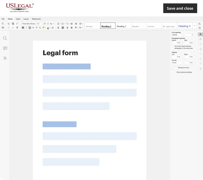
Make edits, fill in missing information, and update formatting in US Legal Forms—just like you would in MS Word.
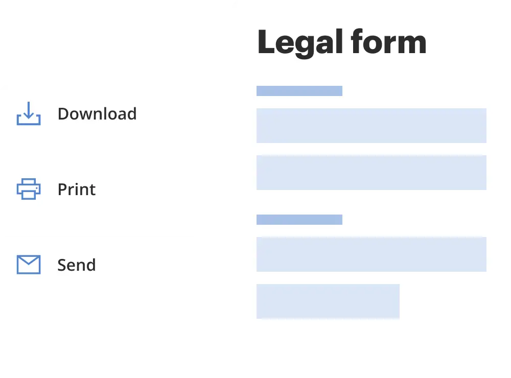
Download a copy, print it, send it by email, or mail it via USPS—whatever works best for your next step.
Sign and collect signatures with our SignNow integration. Send to multiple recipients, set reminders, and more. Go Premium to unlock E-Sign.

If this form requires notarization, complete it online through a secure video call—no need to meet a notary in person or wait for an appointment.
We protect your documents and personal data by following strict security and privacy standards.
Looking for another form?

Form popularity
FAQ
So for time we would type in an equal. Sign then 6 forward slash which is the division sign in ExcelMoreSo for time we would type in an equal. Sign then 6 forward slash which is the division sign in Excel. And then 12 because there are 12 months in a year.
Fortunately, Excel can be used to create an amortization schedule. The amortization schedule template below can be used for a variable number of periods, as well as extra payments and variable interest rates.
Open the Schedule template in Google Sheets At the top of the page, you'll see a section called “Start a new spreadsheet” with several different options to choose from. From here, you'll click “Template gallery” at the top right-hand corner of this section.
Example of Amortization In the first month, $75 of the $664.03 monthly payment goes to interest. The remaining $589.03 goes toward the principal. The total payment stays the same each month, while the portion going to principal increases and the portion going to interest decreases.
Fortunately, Excel can be used to create an amortization schedule. The amortization schedule template below can be used for a variable number of periods, as well as extra payments and variable interest rates.
Calculate simple interest by using the formula I = Prt. In this formula, “I” equals the interest amount, “P” equals principal (the starting balance), “r” equals the interest rate and “t” equals the number of time periods.
If you have an annual interest rate, and a starting balance you can calculate interest with: =balance rate and the ending balance with: =balance+(balancerate) So, for each period in the example, we use this formula copied down the table: =C5+(C5rate) With the FV function The FV function can...
Enter a formula that contains a built-in function Select an empty cell. Type an equal sign = and then type a function. For example, =SUM for getting the total sales. Type an opening parenthesis (. Select the range of cells, and then type a closing parenthesis). Press Enter to get the result.
If you have an annual interest rate, and a starting balance you can calculate interest with: =balance rate and the ending balance with: =balance+(balancerate) So, for each period in the example, we use this formula copied down the table: =C5+(C5rate) With the FV function The FV function can...
After creating your data table, the next step is to input your function into the cell where you want to calculate the interest. To do this, click on the cell and navigate to the formula bar above the column names. In that bar, enter =CUMIPMT(rate,nper,pv,start_period,end_period,type).